Thus the estimate of ![]() can be constrained in both smoothness and
monotonicity. A smoothness constraint may be formulated
by appending
can be constrained in both smoothness and
monotonicity. A smoothness constraint may be formulated
by appending ![]() extra rows to
extra rows to ![]() and the same
number of extra zeros to the end of
and the same
number of extra zeros to the end of ![]() ,
where
,
where ![]() is the length of the appropriate
smoothness filter,
is the length of the appropriate
smoothness filter, ![]() , and then
solving (12).
The extra rows appended to
, and then
solving (12).
The extra rows appended to ![]() are constructed as follows:
Let
are constructed as follows:
Let
![]() denote the portion appended to
denote the portion appended to ![]() ,
and create
,
and create
![]() as a toeplitz matrix in which the first
as a toeplitz matrix in which the first ![]() elements
of the first row are the filter coefficients, and the remaining
rows are appropriately shifted versions of the coefficients:
A_s =
[
elements
of the first row are the filter coefficients, and the remaining
rows are appropriately shifted versions of the coefficients:
A_s =
[
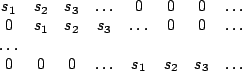
]
In order to achieve smoothness, the filter needs to be a
highpass filter.
(The intuition for this comes from the fact that by ``looking''
at the function through a highpass filter,
this makes it ``expensive'' for the curve
to have high frequency (non-smoothness) content since the
right hand side vector for this portion of the matrix equations is zero.)
The simplest filter is a three-tap filter
![]() for which
the effect of appending the corresponding
for which
the effect of appending the corresponding
![]() to
to ![]() is to impose a penalty for
nonzero second derivatives (inflection) of the curve
is to impose a penalty for
nonzero second derivatives (inflection) of the curve ![]() .
The amplitude,
.
The amplitude, ![]() , of the filter, determines
how heavily the smoothness constraint is weighted.
Additionally, a monotonicity constraint may be imposed using
Quadratic Programming (QP).
, of the filter, determines
how heavily the smoothness constraint is weighted.
Additionally, a monotonicity constraint may be imposed using
Quadratic Programming (QP).
Examples of determining the response function, ![]() , from two differently
exposed images, are shown in Fig 2(a).
, from two differently
exposed images, are shown in Fig 2(a).