Abstract

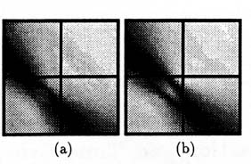
We propose a novel transform, an expansion of an arbitrary function onto a basis of multi-scale chirps (swept frequency wave packets). We apply this new transform to a practical problem in marine radar: the detection of floating objects by their "acceleration signature" (the "chirpyness" of their radar backscatter), and obtain results far better than those previously obtained by other current Doppler radar methods. Each of the chirplets essentially models the underlying physics of motion of a floating object. Because it so closely captures the essence of the physical phenomena, the transform is near optimal for the problem of detecting floating objects.
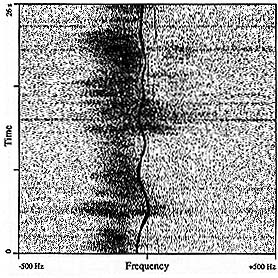
    Besides applying it to our radar image processing interests, we also found the transform provided a very good analysis of actual sampled sounds, such as bird chirps and police sirens, which have a chirplike nonstationarity, as well as Doppler sounds from people entering a room, and from swimmers amid sea clutter.
    For the development, we first generalized Gabor's notion of expansion onto a basis of elementary "logons" (within the Weyl-Hiesenberg group) to the extent that our generalization included, as a special case, the wavelet transform (expansion in the affine group). We then extended that generalization further to include what we call "chirplets". We have coined the term "chirplet transform" to denote this overall generalization. Thus the Weyl-Hiesenberg and affine groups are both special cases of our chirplet transform, with the "chipyness" (Doppler acceleration) set to zero.
    We lay the foundation for future work which will bring together the theories of mixture distributions (Expectation Maximization) and our "Generalized Logon Transform".

Keywords: Time-Frequency, chirplet, chirp, logon, Gabor, wavelet, Doppler, Expectation-Maximization.

Gabor's "Logon" Paradigm
Gabor proposed an expansion of a signal onto a set of bases which he illustrated by way of "logons", which are portions of a Time-Frequency (TF) space¹ He showed that an arbitrary signal can be decomposed onto a set of functions which are all just modulated versions of a single Ganssian

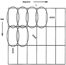
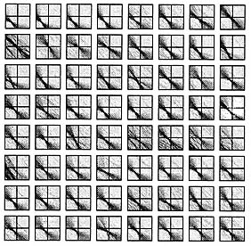
Figure 1: Logon representation of a "complete" set of Gabor bases of relatively long duration and narrow bandwidth. We use the convention of frequency across and time down (in contradiction to musical notation) since our programs that produce, for example, sliding window FFTs, compute one short FFT at a time, displaying each one as a raster line as soon as it is computed.

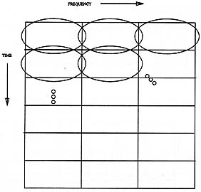
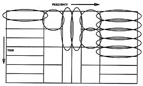
envelope. This notion is known formally in the physics literature as the Weyl-Hiesenberg group. (The "sliding window Fourier transform" belongs to the Weyl-Hiesenberg group since we can think of the bases as being modulated versions of one parent window.) Gabor emphasised the use of a Gaussian window, since it minimises the uncertainty product tf (provided that these support measures are quantified in terms of the root mean square deviations from their mean epochs[2]). The time-frequency logon diagrams, depicted in figures 1 and 2 show how the Gabor function bases cover the time-frequency space, and how we can trade frequency resolution for improved temporal resolution. Gabor originally used rectangles to designate each of these elementary signals. If each of these rectangles were a pixel, and its brightness was set in accordance with the appropriate coefficient in the signal expansion (for example by replacing the rectangle with a dither pattern), the logon diagram would be a density plot (image) of the TF distribution.

Figure 2: Logon representation of a complete set of Gabor bases of relatively short duration and broad bandwidth. We have traded off frequency resolution in order to get better temporal resolution.

1.1 The wavelet transform within the logon paradigm
The wavelet transform may be thought of as breaking up the signal into a set of affine-shaped bases, as illustrated in figure 3. In all our TF figures we show frequency on a linear scale. Thus we can readily see that the aspect ratios of the bases are proportional to the distances from the f = 0 axis. The aspect ratios are still constrained, but the constraint is different. Instead of the constant size constraint of the Weyl-Hiesenberg type expansion, we have a constant "Q" (ratio of bandwidth to center frequency) constraint.

2 "Wavelets" and Wavelets
In our development of a Generalized Logon Transform (GLT), we first removed the constraints of constant aspect ratio or constant Q; we expanded arbitrarily onto a basis of "wavelets" of varying shape, with the only constraint being that each "wavelet" be a Gabor function.br>     In the past, the term "wavelet" often denoted any arbitrary basis function which acted as a bandpass filter (when used as a convolutional kernel). More recently, however, the term wavelet has been used to denote a basis function of constant shape (from an affine group of translates and dilates of one mother wavelet). Indeed, in the earlier papers, the term "wavelets of constant shape" was often used to denote the affine basis explicitly. Whenever the word "wavelet" appears in quotes, we mean "wavelet" in the wide sense: any ephemeral burst of energy, finite in physical support (which includes bases in both the Weyl-Hiesenberg and the affine spaces).

Figure 3: Logon representation of the set of basis functions corresponding to a wavelet transform. Note the two-sided spectrum (zero in center), since we generally use wavelets which lie in the Hardy space (analytic wavelets). These complex wavelets do not suffer from mirroring in the f = 0 axis. Daubechies has shown that we cannot have a set of orthonormal wavelet bases which lie in the Hardy space, so we limit ourselves to non-orthogonal frames.

3 Chirps
A pure tone is given by:

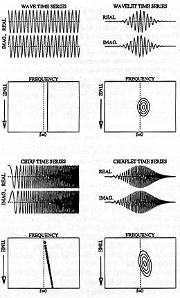
where j = and f_c is a constant (the frequency of the tone in cycles per second).br>     A chirp is a swept frequency where the instantaneous frequency varies with time. Chirps are most familiar as the sound made by a bird or a bat.
    Initially, suppose we have a linear chirp given by:

Physically, the notion of instantaneous frequency is somewhat abstract [Carson,1922], as we know that the frequency can only be measured to within a certain precision, so if the time evolution of the chirp frequency were measured, it would be found to lie along some fuzzy line made of estimated points in TF space, where a regression could be applied to estimate the slope.

4 The Chirplet at a Single Scale
Generally we window the chirp so that it will be finite in extent. We may use the Ganssian window²

Figure 4: Relationship between wave, "wavelet", chirp and "chirplet", in terms of time series and magnitude Time-Frequency (TF) distributions.

but with one small modification. Since we desire unit L2 norm, we instead let

For now, we leave the dilation parameter c constant.
    We then have a chirp "wavelet" for which we have coined the term "chirplet". Figure 4 shows that the relationship of a chirplet to a chirp is analogous to that of a wavelet to a wave. Asymmetric wavelets axe nothing new; Daubechies has shown that eliminating the constraint of symmetry makes

Figure 5: Single scale chirplet transform of an ideal chirplet. Expanding a chirp onto a basis of chirps results in a spread which illustrates a fundamental resolution limit in space akin to the Hiesenberg uncertainty relation in TF space.

it easier to form an orthonormal set, but here we have deliberately introduced a specific form of asymmetry and will exploit this structure in what follows.
    We define an expansion onto chirps:

Where x(t) is an arbitrary time series, and the two dimensions in the transform domain are the slope of the frequency rise a and the center frequency b. We call this space "bowtie () space" since one of the chirp bases itself, expanded onto a basis of chirps has bowtie-shaped contours (see figure 5) in this a and b space. Any signal can be expanded as a weighted sum of these chirps. We can think of this process as fitting the distribution to a number of -shaped "centers" much as we had fit the distributions by somewhat elliptical (almost bivariate Gaussian) centers in TF space. Pure tones are characterised by bowties on the y axis (the middle line a = 0). Downchirps are to the left of this line, while upchirps are bowties situated in the right-hand half of this space. The fact that the chirplet transform of a chirplet itself is not a perfectly sharp spike is a consequence of the overlap of the bases and the fundamental resolution limit inherent in any transform.
    Once we specify the scale (number of samples) and the window function, we may characterise the chirp in one of two ways:

• By specifying the chirpyness (rate of change of instan\-taneous.frequency) a and the center frequency (average instantaneous frequency) b.
• By specifying the beginning frequency f_beg = b - a and the ending frequency f_end = b + a. (For simplicity we have assumed the window essentially starts at time t = -1 and ends at time t = +1.)

4.1The Nyquist boundary problem
Ideally we would like our transform to have nice "Manhattan'' rectangular boundaries for convenient viewing on a video display. When we parameterize the chirplet space in terms of slope (rate of frequency change) and intercept (average frequency), we have an inconvenient shape of bound\-ary. The Nyquist limits dictate that the "chirpiest" of chirps goes from a fractional frequency of -1/2 to 1/2 (or +1/2

Figure 6: Single scale chirplet transform of a pure tone. Here we parameterize the chirplets by starting frequency and ending frequency.

down to -1/2). This chirp will lie on the b = 0 axis, as far to the right as possible (or as far to the left as possible). But then a chirp which has the same value of a, but a non-zero intercept (for example one going from fractional frequency -1/4 to 3/4), will violate the Nyquist limit and give rise to aliasing in frequency space.
    It turns out that the Nyquist boundary in the (a, b) space is diamond-shaped, and so we can overcome the problem by just tilting the space 45°. Figure 6 shows the chirplet transform of a signal which is itself a special case of a chirplet, namely a pure tone (modulating a Ganssian envelope). We define the starting frequency as the frequency of the wave at the beginning of the window, and the ending frequency as the frequency at the end of the window. When we use Gaussian windows, we generally define the window boundaries in terms of the 3 points.
    In this single-scale "chirplet snapshot" we fix both the mean epoch location and the physical support (resolution), and vary the center frequency and chirpyness (where we have used our new display format which provides explicitly f_beg on the across (left.to right) axis and f_end on the up axis).
    The center of this chirplet snapshot gives a measure of how strong the chirp component from 0 to 0 (the DC component) is. The value at coordinates (0,1/2) gives the strength of the component of a chirp going from a fractional frequency of 0 to 1/2. Now, any points on the line y = x correspond to pure tones. Points in the upper left half (above this line) correspond to coefficients of upchirps; those to the lower right correspond to downchirps.
    We allow considerable overlap in the bases, and allow the slant of the individual logons to vary in a somewhat continuous fashion. (We have also tried adapting[3]the bases; an adaptive "wavelet" or chirplet transform allows accurate representation with a very small number of coefficients.)

5 Multi-Scale Chirping "Wavelets" (GLT basis functions)
We propose a basis of multi-scale chirps. Of course the Ga-bor functions (of both the Weyl-Hiesenberg and the affine groups) are just special cases, where the chirp rate is zero (the beginning instantaneous frequency equals the ending instantaneous frequency), corresponding to constant velocity

(zero acceleration) in terms of Doppler. Our previously described "bowtie" space is also a special case of this generalization, where the scale is fixed constant.
    There are 5 free parameters in each of our basis functions:

• Temporal location: location of the mean epoch within the time series being analysed.
• Physical support, t, otherwise known as the effective pulse width or scale. t (the parameter c in equations 6 and 7) is usually measured in terms of the RMS deviation from the mean epoch (the "second-order moment" ).
• Center frequency; the mean epoch in Fourier space.
• "Chirpyness"; the rate of change of the instantaneous frequency. If the chirpyness is zero, we have a pure Gabor function.
• Relative phase: the phase between the Ganssian envelope and the chirp it is modulated by.

    If we are only looking at the magnitude or power distribution of the GLT, we can ignore the last parameter because all the GLT bases are complex and lie in the Hardy space (their imaginary parts are equal to the Hilbert transforms of their real parts). Because these functions are analytic, the contribution due to one of the bases is very insensitive to the relative phase.
    Chirps correspond to slanted logons which can fill the time-frequency space completely.
    We can expand any arbitrary signal onto a basis of up-chirps, downchirps, or a mixed basis of upchirps, downchirps, and ordinary Gabor functions which all show up as nearly elliptical contours (having equal areas) in time-frequency space³ but with different slants (orientations) and aspect ratios.
    By tilting the logons, we can simultaneously increase the support in both domains, without losing optimality in cojoint resolution, along a tilted set of axes ("s/" for slant), where t_slf_sl is still 1/2.

6 Application of the GLT to Detection of Floating Objects in Ocean Based Radar
We apply our transform to radar image processing for the identification and tracking of floating targets such as iceberg fragments and smaller boats, which pose a collision hazard to navigating vessels. In particular small pieces of icebergs ("growlers"), about the size of a grand piano, can do extensive damage to a vessel, but axe too small to show up on conventional marine radar systems.

---

³The approach of Slepian[4], who used functions which are truly rectangular in TF space, can be extended to chirps. Our "Slepian chirplet" then represents an ideal parallelogram in TF space. We may then apply Thomson's method of multiple windows[5] to our chirplet paradigm.

6.1 Fourier based Doppler processing
Since a strong component of the radar backscatter from the target will be "in phase with itself", due to the cohesiveness of the target, we can rely on the Doppler characteristics of the returns. Much work has been done using classical Fourier based techniques to characterise floating targets[6, 7]. These techniques rely on the fact that the targets give rise to backscatter which has narrow spectral width. An object at rest has a narrow Doppler spectrum, centered at zero. An object moving at a constant speed has a narrow Doppler spectrum centered at the corresponding Doppler frequency. What we propose, is a novel way of looking at the time evolution of this Doppler spectrum.

6.2 Underlying physics of motion
If you have ever watched a cork bobbing up and down at the seaside, you would notice that it goes around in a circle with a distinct periodicity^4.
    It goes up and down, but it also moves horizontally. Looking out at a target with the radar, we see the horizontal component of the motion which is the Hilbert transform of the up and down motion. Thus the range variation of the object (a time series formed by sampling the "distance" between the radar and the object) has the same periodicity. This near sinusoidal periodicity in the range motion of the target shows up as a "squiggle" in TF space as shown in figure 7. The target may be characterised by this snake like ridge or skeleton. (The term "snake" is due to Terzopoulos[9], who develops a means of dynamically tracking contours, in an arbitrary image, with energy minimising splines.)

6.3 Projections of the chirplet as indicators of Doppler evolution of floating objects
Two-dimensional slices through the CLT space allow us to view it on a video display or printed page. We look at a hyperplane passing through the space. If we pick the axes center frequency and scale, we can immediately recognise a target based on the constancy over all scale space (see figure S).
    Note also that at higher frequencies, the scale is higher, the loci of these points indicate an anti-fractal trend (fractal behaviour usually gives rise to an affine characteristic: larger scales for lower frequencies, in other words, "constant" Q).

Figure 7: Sliding window FFT of "growler" (small iceberg fragment)

floating object, (compare figures 9 and 10), but in an even more pronounced way. Furthermore, we have an explicit measure of the target's "chirpyness". In other words, we can see the acceleration signature of the target, and use this information to fit to a physical model. Such physical constraints are useful for verification and also for target tracking. We will refer to this particular choice of two variable parameters as a single-scale chirplet snapshot. The term single-scale refers to the fact that all the bases have the same duration, or physical support (in this case one second). The word snapshot refers to the fact that we are glancing at the target at a particular "instant" (over a short interval of time) and are not tracking the temporal evolution of the acceleration signature.
    As mentioned earlier, a diagonal slice through the single-scale chirplet snapshot (along the line f_beg = f_end)is just the Fourier transform (with the same window as that used in

Figure 8: Slices through GLT, along the hyperplane defined by f_beg = f_endfor a fixed temporal center defined by t_o = constant. (a) With floating object (growler) present. (b) With sea-clutter only.

Figure 9: Chirp Logon Transform of one second of time series from range cell with growler. The location of concentration of most of the density shows us that an object, which accelerated from about 0m/s to about 0.9m/s during the one second glance, was present.

the chirplet) of the original time series. In figure 11 (a) we show this slice. If, however, all we want is one free rameter, we are far better off to take the slice through the "bowtie" center. In figure 11 (b) we see that the "Average Instantaneous Frequency" spectrum (AIF spectrum) is much sharper than the Fourier spectrum.

7 Classification using the GLT
Problem: Given 1/2 second of radar return from a particular range cell, decide whether or not a floating object is present (2 class problem).
    To train the classifier, we use 256 single-scale GLT snapshots, (each one formed from 512 complex samples). We evaluate the performance based on a testing set which is independent of the training set.

7.1 GLT snapshot features
    We draw 3 features from each GLT snapshot:

• "Entropy": the sum of pixel brightnesses times the logarithm of these brightnesses. (The word is in quotes, because entropy usually deals with random distribu\-tions). If all pixel brightnesses are equally probable, we get a high "entropy". This quantity was high for GLT snapshots which contained no target, and low for those with targets.
• Extent: Target GLT snapshots are much more compact, clustered about the mean epoch of the energy distribution. Those of clutter, on the other hand, are much more spread out. We fit a bivariate Gaussian

Figure 10: Chirp Logon Transform of one second of time series from range cell with sea clutter only.

Figure 11: Slices through the single-scale chirplet snapshot: (a) A slice along the diagonal is just the Fourier spectrum. (b) When we shift over to the center, however, we obtain a much sharper peak.

distribution to the data Although the logon is no longer Gaussian in the GLT space, the Gaussian fit allows us to quantify the spread by the determinant of the covariance matrix, |S|. These values correspond to the second-order moments of the distribution.

• Slenderness: The ratio of largest to smallest eigenval-ues of S. We have observed that targets give rise to slender "blobs".

7.2 Classification Results
The classification results, using 6 different methods, are presented in Table 1.

We have used Fishers Linear Discriminant (FLD)[10] in preference to Principal Components Analysis (PCA) which only looks at the variance of the features, and requires scaling in accordance with an assumed a priori knowledge of the feature importances.

7.3 The Neyman-Pearson Paradigm
We would rather have a false alarm than miss a target, so the risk function is not symmetric. In table 1, however, for simplicity, we have assumed a (binary) symmetric risk function. Binary risk implies equivalence between the Maximum A posteriori Probability (MAP) classifier and the Bayes classifier. Symmetry, however, can be dealt with by either providing Receiver Operating Curves (ROCs) or more simply, by differentiating between type 1 errors and type 2 errors, by means of a confusion matrix.
    In our confusion matrices, the first row represents feature vectors known explicitly to belong to class 1, while the second row represents those known to belong to class 2. The off diagonal elements represent the errors, and the rows sum to 100%. The upper right entry, for example, represents the fraction of those feature vectors which we know belong to class 1, but which were classified as belonging to class 2. The ordering of the 6 confusion matrices appearing in table 2 is the same as the ordering of the raw performance figures appearing in table 1. All values axe rounded to nearest integer percentage (2 significant figures).

7.4 Weighted k-Nearest Neighbours
Finally, we propose a variant of kNN, Weighted k-Nearest Neighbours (WkNN), where we take a weighted average of the class decisions for each of, say, k, nearest neighbours. By using a decaying weighting function, we apply more confidence to the nearest neighbour than the second nearest, and more to the second than to the third, and so on. The weights were set inversely proportional to the Euclidean distances

from the corresponding exemplars. If, for example, the distance from the input feature vector to the "winner" was just a bit less than the distance to the "runner up", the first and second weights would be nearly equal. If, on the other hand, the winner was much closer than all the others, its class would be weighted very highly compared to the classes of all the others.
    WkNN has another additional advantage: it gives a Neyman-Pearson output by providing, explicitly, a real valued class decision. This feature is useful when Receiver Operating Curves (ROCs) are desired.

8 Skeletonisation and Time Evolution of the GLT Snapshot
A single GLT snapshot captures time evolution of the Doppler spectrum, but we can still do better by looking at the time

Figure 12: Successive single-scale chirplet snapshots of a floating iceberg fragment. The time evolves from left to right, starting at the top row (same ordering as in a TV raster scan). Since the growler is bobbing up and down in the waves, it will be hidden completely from the radar at times. The snapshot in the sixth row, first column, resembles clutter because the growler is hidden at this time. Note also the clockwise elliptical locus.

evolution of the GLT snapshot itself. The images in figures 9 and 10 were just "snapshots" of the GLT evaluated at a fixed temporal center. If we move the center epoch of the bases through the data, we can see, basically, a single prominent elementary chirp, moving around on an elliptical locus. (We developed software to display a "movie" or animation of the successive GLT snapshots in sequence on the computer screen. 64 of these snapshots appear in figure 12.) We have coined the term "hypermatrix" for this structure, which we say has 64 "pages", and the rows and

columns of each page make up the image. In figure 13 the loci of this movement are shown, for two different sets of 64 snapshots, projected onto the temporal center axis. (By projection, we mean the average, summing over all pages of the hypermatrix, to reduce three "index dimensions" to two.)

Figure 13: Projections of the helical paths of the "bowties" onto the temporal center (time) axis. The elliptical "holes" indicate the empty regions down the centers of these helical loci. (a) Recorded data b98, range 25. (b) Recorded data b97, range 27.

    If we visualise this path in three dimensions, we have a helix. A slice through this hypermatrix, along the plane f_beg = f_end results in the time-frequency squiggle we saw in figure 7.
    We were able to do much better by tracking this helix in GLT space, than by using single GLT snapshots alone. In · other words, keeping a memory of the previous GLT snapshots, we predicted where we would expect the next peak epoch to be. Feeding this previous information into the classifier gave a result of 98% performance. This process requires "bootstrapping" the classifier (allowing it time to "latch on").

9 Current Research
    The chirplet transform we have so far described assumes a model of piecewise constant acceleration. Within GLT space, conventional Doppler radar treats the helical skeleton as piecewise constant, whereas the GLT treats it as piecewise linear. We may extended the chirplet bases to piecewise quadratic, or piecewise cubic, but instead we developed a set of bases which chirp to describe a sinusoid in TF space (a true piecewise sinusoidal helix in GLT space).
    We then extended the approach of Stephane Mallat (wavelet maximal11]) to our chirplet paradigm, using optimization techniques to select a few-well chosen bases corresponding to local maxima of the sinusoidal chirplet expansion. We showed that a signal could be reconstructed exactly, given only these local maxima.
    We have extended the Expectation Maximization (EM) theory, which is already well known for its use in approximating an arbitrary mixture distribution by a weighted sum of Gaussians, into the realm of Time Frequency space. The "EM centers" (positions of the ellipses) become the center frequency and temporal center. The aspect ratio becomes the tradeoff between duration and bandwidth, and the tilt of the ellipse is just the chirpyness. We can display the

process on the screen as either constant area ellipses moving and twisting to fit the TF distribution, or as bowties moving around in the chirplet space.
    We are working on a Radial Basis Functions (RBF) neural network classifier, where our Logon Expectation Maximizer (LEM) will become its front end. We may then design an optimal classifier based on approximation theory[12] where we are developing an approximation to this approximation theory, since we cannot have an exact Time Frequency distribution[13].

References

[1] Ingrid Daubechies. The Wavelet Transform: a method for time-frequency localization. Appears as a chapter in Advances in Spectrum Analysis and Array Processing: Simon Haykin, Editor, 1991.

[2] D. Gabor. Theory of communication. J. Inst. Elec. Eng., 93:429-456, 1946.

[3] Steve Mann and Simon Haykin. An Adaptive Wavelet Like Transform. SPIE, 36th Annual International Symposium on Optical and Optoelectronic Applied Science and Engineering, 21-26 July 1991.

[4] D. Slepian, H. Pollack, and H. Landau. Prolate spheroidal wave functions, fourier analysis and uncertainty. Bell System Technical Journal, 1961.

[5] D. Thomson. Spectrum estimation and harmonic analysis. Proc IEEE, Sept. 1982.

[6] B.W. Currie, S. Haykin, and C Krasnor. Time-varying spectra for dual polarized radar returns from targets in an ocean environment. IEEE Conference proceedings RADAR90, Washington D.C., May 1990.

[7] S Haykin, C Krasnor, Tim Nohara, B Currie, and D Hamburger. Coherent dual polarized radar studies of an ocean environment. IEEE Transactions on Geosciences and Remote Sensing, Feb 1991.

[8] Gary Mastin, Peter Watterberg, and John Mareda. Fourier synthesis of ocean scenes. IEEE CG&A, 1987.

[9] Michael Kass, Andrew Witkin, and Demetri Terzopou-los. Snakes: Active Contour Models . Academic Publishers, 1987.

[10] Richard Duda and Peter Hart. Pattern Recognition and Scene Analysis. John Wiley and Sons, 1973.

[11] Stephane Mallat. Compact image representation from multiscale edges. Submitted to 3rd International Conference on Computer Vision, 1990.

[12] Tomaso Poggio and Federico Girosi. Networks for approximation and learning. Proc. IEEE, 1990. Sept.

[13] D Lowe. Joint representations in quantum mechanics and signal processing theory: why a probability function of time and frequency is disallowed. Royal Signals and Radar Establishment, 1986. report 4017.